My Small World

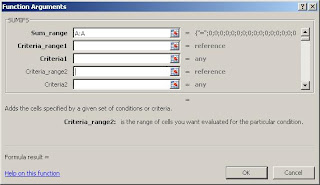
We already know the primary challenge of using SUMIF or SUMIFS i.e. unable to sum more than a single column or row as a sum range. Many of us in the course of our excel usage may have experienced that SUMIFS has a bigger disadvantage when used across workbooks i.e. the source workbook should be open inorder to enable to computation in the destination workbook. If the source workbook remains closed, the result in the destination workbook will be "#VALUE". In my previous post , the alternative suggested not only does overcome the  "#VALUE" challenge but also allow users to sum a larger range.  In this post, I was able to decipher yet another alternative. I'm sure expert users may already be using this however to help other users, this post can be a ray of hope. We may have used the SUMPRODUCT function to calculate weighted average. Extrapolating the usage of SUMPRODUCT with condition or conditions can help you achieve the SUMIFS goal.  Syntax:  =SU...

I've had few posts earlier on few excel shortcuts. Navigation powered by "Ctrl" in Excel Shortcut to insert current date in a cell Shortcut to AutoFilter So, here I am, back with some more interesting shortcuts which will make your excel spreadsheet experience simpler. Let me start with some "CTRL" combinations which will be very handy for formating cells to match your requirements: CTRL + 1 : Opens the "Format Cells" dialog box CTRL + 2 : is to make the contents of the cell BOLD (this is a toggle key, to unbold use same CTRL + 2) CTRL + 3 : is to make the contents of the cell ITALICS (this is a toggle key) CTRL + 4 : is to underline the contents of the cell (this is a toggle key) CTRL + 5 : is to strike through the contents of the cell (this is a toggle key) CTRL + 9 : is to hide the entire row (to unhide use SHIFT + CTRL + 9) CTRL + 0 : is the hide the entire column (to unhide use SHIFT + CTRL + 0) CTRL + ~ : is to show or...

Ever wondered while using "SUMIF" function, the sum range cannot be more than one column!!  This indeed is a big drawback while using a large data set where you need to sum matching certain conditions. I often end up using multiple sumif with "+" which makes the formula very long. So was thinking of some alternative that can make life easier. Thanks to the search engines these days, I did come across a workaround. Refer to the above image: In the above example, I have a table with 4 columns where H1 and H2 are identifiers. H3 and H4 is the data which needs to be summed up. Condition 1 (alternative for SUMIF): I need to sum values of H3 and H4 where the identifier H2 is "Y". The formula will be =SUM(IF(B2:B5=B9,C2:D5)) followed by Ctrl + Shift + Enter which will make it a array formula. The final formula will look like this:  {=SUM(IF(B2:B5=B9,C2:D5))} Condition 2  (alternative for SUMIFS) : I need to sum values of H3 and H4 where the ...

VLOOKUP syntax We often encounter "#N/A" while using VLOOKUP function to compare two lists. One of the most common problems that give rise to this error is extra spaces either to the end or to the beginning of the string. What's the way out? The simplest way out is to use "TRIM" function as a sub function. Example While trying to use VLOOKUP in the normal course, the result will be "#N/A", whereas with TRIM nested in the VLOOKUP function will give the positive result. (TRIM function removes the unwanted spaces in the beginning and end of a string.)

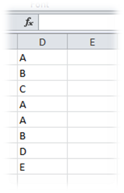
Though MS Excel today allows to easily eliminate duplicate values in a list, have you ever tried to identify the number of entries that gets repeated in an excel list? In the above example, we can identify the repeat entries using "COUNTIF" function. Option 1 formula: =COUNTIF($D$1:D1,D1) Explanation: This formula counts the occurrence of the value in the list i.e. on the first occurrence, the result will be one and on the second it will be 2 and like wise. (see the figure below) Option 2 formula: =COUNTIF($D$1:$D$8,D1) Explanation: This formula counts the total number of repetitions. If an entry appears thrice in a list, then the result will be 3 in all the occurrences of that entry. (see the figure below) So start using whichever is convenient to you... :)

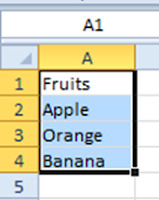
Have you ever wondered if we can have a dynamic drop down list i.e. a drop down using data validation that gets updated automatically with any change in the source of the drop down... I often faced problems having a dynamic drop down list but ultimately I was able to find a solution to my problem. Step 1: Format the source list as a table and name the table (here I've named the table as "Fruits") Step 2: Go to Formulas -> Name Manager and click on New Define any name in the dialog box In the example, I've named it as "Names". Then click on Refers to field and select the table in the excel sheet. The refer to will appear as =TableName[ColumnName] Step 3: Now create the drop down list using data validation and mention the source as the name you defined. In this case "Names" Here you go. The drop down list hence created is dynamic. Any addition or deletion in the source table of the drop down ...

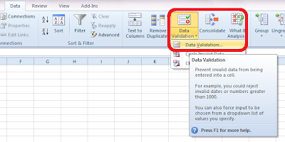
In a series where I would like to present on the power of "Data Validation" option in MS Excel, the first and commonly used function is creation of a drop down list in a cell. We often come across situation where we feel the necessity of having a drop down list in a worksheet where the inputs are predefined and the user gets ready option to populate the cell. The easiest way to create such a dropdown is typing out the list values in the data validation -> list option. Step 1 : Go to Data -> Data Validation -> Data Validation...   Step 2 : Select "List" option in the "Allow" drop down box   Step 3: Write down the desired list values seperating them with comma in "Source" box Result: You get the drop down with the desired options in the intended cell What if you intend to create a long list where the entries are too much? Don't worry, excel offers you solution for this as well. Instead of the "Ste...

I had been wondering how can I get a complete stock of the directories as well as contents on my system. In this endeavor Google came to my rescue and directed me to a post where I could find a DOS command to print the directory structure in Windows environment. For Example: If you need to know the contents of the C drive, then go to the command prompt and type  "dir C:\ /s >output.txt" where: dir -  the dos command for displaying the directories C:\ - the location of which you want the directory structure /s - the dos command extension for displaying not only the directories but the files as well >output.txt - refers to the name of output file (in this case output.txt) which will be placed at the root of the folder where the command is getting executed. In case you want the output to your specified location, then include the complete path of the destination after ">". Source:  http://superuser.com/questions/258287/what-is-a-good-...

(in continuation of my earlier post: " Custom Validation in Excel ") Today I seriously recognised the power of data validation. I was stuck in a situation wherein I had to create a template wherein the user needs to enter a date, however it the date cannot be a Saturday or a Sunday. After a brief "R&D", I realized using "data validation" was the apt option. Go to Data -> Data Validation In the dialogue box which pops up, choose "Custom" from the drop down under Settings -> Validation Criteria -> Allow In the new field "Formula", just enter the criteria you want to achieve. In my case, I used "=WEEKDAY(A2,2)<6" Then, you may click on the "Error Alert" tab and may put any customized error alert like the picture below: So, now the desired cell is validated and user can only enter a weekday. Another, popular validation that I often use is the "List" wherein one can easily cr...

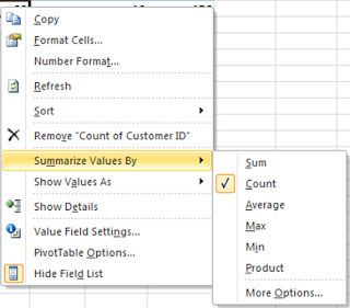
Excel 2007 onwards, playing around with Pivot Table has become even more user friendly. Pivot was seemingly a tool preferred by advanced users of excel but today its a child's play :) Extended options over right click has made this a must use tool for all users who are required to handle a reasonable amount of data. For eg: "Summarize Values By" on right click gives you the option to summarize data by sum or count or average or to choose from all available options. Earlier, one had to be conversant with the options to actually use it. "Show Values As" on right click allows to apply calculations to the data area. Microsoft is making more and more features available for average / less than average users who actually are keen to use the features. Lets all of us make use of this. Note: In case my readers want, I can explore on writing a basic step by step guide on basics of Pivot Table!

We often tend to encounter instances while using formulae performing day to day operations where the formulae results in an error. Often, some basic users prefer manually correcting those errors and so advance users go one step ahead using a combination of "IF" & "ISERROR" functions. Even I'm one of those users who prefer using the "IF" & "ISERROR" combination until I came across the "IFERROR" function. Syntax: IFERROR(value,value_if_error) According to Microsoft, "IFERROR" evaluates  #N/A, #VALUE!, #REF!, #DIV/0!, #NUM!, #NAME?, or #NULL! type of errors. Say: Cell A1 contains a numeric value and Cell A2 contains 0 as value. You intend to perform a simple operation A1 divided by A2 (=A1/A2). In our example, the result would be #DIV/0!. Now, lets redo this simple division using "IFERROR" function. The formula can be written as "=IFERROR(A1/A2,0)" wherein the formula would asses that if the...

In Excel 2007 and 2010, there is a feature called AutoRecover that saves your open workbooks at regular intervals. In the event of a power failure or computer crash or freeze up, this can help you recover your unsaved work. This feature is turned on by default and is hardly noticeable as it happens in the background. However, you may notice AutoRecover saving files, and may even get annoyed by it, if you have one or more large workbooks open, as it could tie you up for 5 to 10 or more seconds. I often have very large workbooks open that contain only reference information (i.e. files that I'm not making changes to) and other workbooks which I don't require to be saved by the AutoRecover feature. To avoid the unnecessary saving of these files, there is an option available to turn off AutoRecover for individual workbooks. Here's how... 1) Click the File tab (2010) or the Office Button (2007); 2) Click Options (2010) or Excel Options (2007); 3) Clic...

A simple subtraction between two date values gives you the number of days between the two days. However, to actually calculate the exact number of days or number of completed months or number of completed years, Excel offers a hidden function called "DATEDIF". Syntax: =datedif(date 1, date 2,criteria), where date 1 is the start date or the older of the two dates date 2 is the end date or the recent date Criteria can be as follows:   "d" - number of completed days between the two dates   "m" - number of completed months between the two dates   "y" - number of completed years between the two dates   "yd" - number of completed days between dates ignoring the year i.e. considering them to be in the same year  "ym" - number of completed months between dates ignoring the year i.e. considering them to be in the same year  "md" - number of completed days between dates ignoring the year & month i.e. considering...

Excel 2007 and 2010 versions allow easy shortcut keys to change the case of the text in any given cell. Proper case (1st letter of every word in upper case) - shift + ctrl + p Upper case (all characters in upper case) - shift + ctrl + u Lower case (all characters in lower case) - shift + ctrl + l Isn't it handy?? Published with Blogger-droid v1.6.7

One of the most frequently used feature of Excel is the autofilter. Most power users tend to use Alt+D-F-F for turning the filter on. Excel gives a shortcut for this... "Shift+Ctrl+L". Shift+Ctrl+L provides the ease of applying or removing filter. This is applicable for 2003 version onwards.

Most of the users are very used to formula like " COUNTIF "or " SUMIF "... Excel offers "S" factor adding spice to these handy formulas...  Sumif: usual syntax is =Sumif(criteria range, criteria, sum range) where you want to sum a given range of cells based on a condition in another range of cells. "Sumifs" acts one step further. The syntax is =Sumifs(Sum range, Criteria range1, criteria1, Criteria range2, criteria2...) and go on to add upto 9 criteria . This is handy when we need to sum a range based on more than one criteria. Similarly, we are quite used to "Countif" formula while counting a given range based on a filter criteria. Just like sumifs, countifs offers the same operation with multiple criteria filtration. Countif syntax: =Countif(Count range, Criteria). The countifs syntax gets changed to =countifs(Criteria range1, criteria1, criteria range2, criteria2....) . This too works upto 9 criteria . Excel really mak...

Want to insert the current date in a cell with just a key stroke...? The answer is simple - "ctrl + ;". This inserts the current system date as per the format configured on your system! Check it out... this is applicable on all versions of excel.

Have you ever tried copying a list where there are multiple hidden rows...? Whats the result?? You will see all the values irrespective of the hidden or visible cells...! Shortcut: Copy the given cell range Press "Alt + C" Press "Ctrl + C" Paste at the desired location (Ctrl + V)   Now see the difference...!  Simple... isnt it?

Have you ever tried combining the contents of two cell... the first thing that comes to mind is "concatenate" (an inbuilt function in excel to combine to strings). The usual syntax for using this function is '=concatenate(Text1,Text2)' where text can be entered directly within quotes or use cell reference i.e. '=concatenate(A1,A2)'.... This may be at time cumbersome to remember. The easy solution... "&" operator which serves the same function as concatenate. The syntax for using "&" is '=(text1 & text2)' where the text is to be entered within quotes. Lets try creating an address book for a company where the email naming concept is firstname.lastname@companyname.com. We just have the list of names i.e. First Name in Column A & Last Name in Column B. Just go to column C and try writing the formula '=(A2 & "." & B2 & "@companyname.com") and just see the merged contents in the new c...

Have you ever tried to create a worksheet where you dont want the user to create duplicate entries...?? Its quite possible in a fairly simple way in MS Excel..! Say you are typing a list of names, where you don't want any name to be repeated once: Step 1: Step 2: Step 3: The formula is a relative formula where it counts the values between the first cell of the column till the current cell to check if the value entered in the current cell is not repeated. Step 4: You may define custom error messages too! Step 5: Copy the first cell to the desired number of cells in the list in order to apply the validation to all the cells in the list. Now try entering few names in the column. Result: So... isnt it easy? Try it out yourself.. and do let me know if this works!!