My Small World

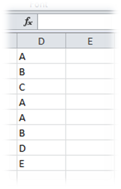
Though MS Excel today allows to easily eliminate duplicate values in a list, have you ever tried to identify the number of entries that gets repeated in an excel list? In the above example, we can identify the repeat entries using "COUNTIF" function. Option 1 formula: =COUNTIF($D$1:D1,D1) Explanation: This formula counts the occurrence of the value in the list i.e. on the first occurrence, the result will be one and on the second it will be 2 and like wise. (see the figure below) Option 2 formula: =COUNTIF($D$1:$D$8,D1) Explanation: This formula counts the total number of repetitions. If an entry appears thrice in a list, then the result will be 3 in all the occurrences of that entry. (see the figure below) So start using whichever is convenient to you... :)

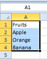
Have you ever wondered if we can have a dynamic drop down list i.e. a drop down using data validation that gets updated automatically with any change in the source of the drop down... I often faced problems having a dynamic drop down list but ultimately I was able to find a solution to my problem. Step 1: Format the source list as a table and name the table (here I've named the table as "Fruits") Step 2: Go to Formulas -> Name Manager and click on New Define any name in the dialog box In the example, I've named it as "Names". Then click on Refers to field and select the table in the excel sheet. The refer to will appear as =TableName[ColumnName] Step 3: Now create the drop down list using data validation and mention the source as the name you defined. In this case "Names" Here you go. The drop down list hence created is dynamic. Any addition or deletion in the source table of the drop down ...

One of the most frequently used feature of Excel is the autofilter. Most power users tend to use Alt+D-F-F for turning the filter on. Excel gives a shortcut for this... "Shift+Ctrl+L". Shift+Ctrl+L provides the ease of applying or removing filter. This is applicable for 2003 version onwards.

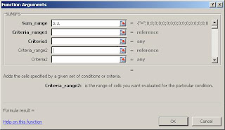
Most of the users are very used to formula like " COUNTIF "or " SUMIF "... Excel offers "S" factor adding spice to these handy formulas...  Sumif: usual syntax is =Sumif(criteria range, criteria, sum range) where you want to sum a given range of cells based on a condition in another range of cells. "Sumifs" acts one step further. The syntax is =Sumifs(Sum range, Criteria range1, criteria1, Criteria range2, criteria2...) and go on to add upto 9 criteria . This is handy when we need to sum a range based on more than one criteria. Similarly, we are quite used to "Countif" formula while counting a given range based on a filter criteria. Just like sumifs, countifs offers the same operation with multiple criteria filtration. Countif syntax: =Countif(Count range, Criteria). The countifs syntax gets changed to =countifs(Criteria range1, criteria1, criteria range2, criteria2....) . This too works upto 9 criteria . Excel really mak...

Want to insert the current date in a cell with just a key stroke...? The answer is simple - "ctrl + ;". This inserts the current system date as per the format configured on your system! Check it out... this is applicable on all versions of excel.

Have you ever tried copying a list where there are multiple hidden rows...? Whats the result?? You will see all the values irrespective of the hidden or visible cells...! Shortcut: Copy the given cell range Press "Alt + C" Press "Ctrl + C" Paste at the desired location (Ctrl + V)   Now see the difference...!  Simple... isnt it?

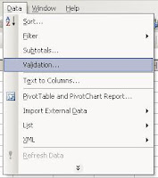
Have you ever tried to create a worksheet where you dont want the user to create duplicate entries...?? Its quite possible in a fairly simple way in MS Excel..! Say you are typing a list of names, where you don't want any name to be repeated once: Step 1: Step 2: Step 3: The formula is a relative formula where it counts the values between the first cell of the column till the current cell to check if the value entered in the current cell is not repeated. Step 4: You may define custom error messages too! Step 5: Copy the first cell to the desired number of cells in the list in order to apply the validation to all the cells in the list. Now try entering few names in the column. Result: So... isnt it easy? Try it out yourself.. and do let me know if this works!!

Have you ever wondered the power of the key "Ctrl" while you are navigating in an excel worksheet or workbook...? The best accelerator key for navigation in excel is "Ctrl"... Move to the beginning of a row                  Ctrl + left arrow Move to the end of a row                          Ctrl + right arrow Move to the beginning of a column              Ctrl + up arrow Move to the end of a column                      Ctrl + down arrow Move to a different worksheets                   Ctrl + Page Up or Page Down Juggle between active workbooks                Ctrl + tab Move to the beginning of worksheet             Ctrl + home Isnt this is a p...

Intermediate to advance users of Excel may be quite familiar with the formula "Round()" where one can round off decimals. Microsoft offers something beyond decimals rounding off by this formula. The usual syntax for rounding off a number is "Round(#ref,1)" where #ref is the cell reference or the number to be rounded off and 1 is the number of decimal places the number needs to be rounded off i.e. if you want two digits after the decimal it should be 2, for one digit it should be 1 and no digits after decimal it should be 0. Have you ever tried using -ve number for rounding off...? Yes..! Using a negative number in the syntax will round of the number to the unit place you desire i.e. " Round(#ref,-1) ". Eg: You wish to round off 123456 to the nearest thousands so the formula would be "Round(123456,-3)" - Result: 123000!! This would be quite handy for the finance and sales people who need to quote rounded figures at various forums..!...

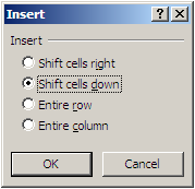
" Ctrl + + " (add rows or columns) and " Ctrl + - " (delete rows or columns) are the easy shortcuts one may remember while adding and deleting rows/columns in Microsoft Excel. Adding rows or columns: If you wish to add rows above the current cell... just press "shift + spacebar" (discussed in my earlier post) to select the current row and then press "Ctrl + +". It will insert a row over the current row. Press "Ctrl + +" repeatedly to insert as many rows. Similarly, "ctrl + spacebar" and then "Ctrl + +" adds a column before the current column. You may try pressing "Ctrl + +" without selecting a row or a column. In such a case, you may get a pop-up (as shown in the image) where you can choose an option of adding a row or a column. Deleting rows or columns: "shift + spacebar" followed by "Ctrl + -" deletes the selected row & "ctrl + spacebar" followed by "Ct...

Here are some keyboard shortcuts for some commonly used tasks. You may find it difficult to remember initially but gradually you would love to remember them. Format as currency with 2 decimal places CTRL + SHIFT + $ Format as percent with no decimal places CTRL + SHIFT + % Apply number format CTRL + SHIFT + ! Apply date format CTRL + SHIFT + # Apply time format CTRL + SHIFT + @ Apply general format CTRL + SHIFT + ~ Apply exponential number format CTRL + SHIFT + ^ Apply outline border to selection CTRL + SHIFT + ; Remove outline border to selection CTRL + SHIFT + _ Note: These shortcut will execute system default formating eg: if the default currency of the system is "$" the currency formated cell will bear "$". If you wish to apply any other formating other than t...

"Sum" formula is one of the widely used formula in Excel. I guess even a novice can do a "sum" calculation in excel. Microsoft offers an easy keyboard shortcut to the formula i.e. " Alt + = ". This command sums the list of values above the current cell. This is equivalent to the  in the standard toolbar in Excel. Isn't it easy??

The common answer to this post would be " Alt + Tab "... a popular windows shortcut. However, there's an easier way to navigate between multiple excel workbooks is " Ctrl + Tab " or " Ctrl + Shift + Tab ". " Alt + Tab " allows switching between all open windows irrespective of application but " Ctrl + Tab " offers the flexibility of switching between open excel files only without disturbing other open applications..! So when you are working on multiple excel files next time... you know which shortcut to use to navigate between open excel files...!  Ctrl + Tab " also help you to navigate between the tabs of any tabbed browser like IE7, Mozila Firefox, Chrome etc.. So now you can remember this more easily...!!

Most of us may have not tried this. We are very much familiar with the world-famous "Ctrl + C" and "Ctrl + V" but have you tried " Ctrl + D " and " Ctrl + R " in excel?? " Ctrl + D " offers the flexibility of copying the content of the cell above to the next cell or a range of cell below. Here you just need to use one action instead of the regular copy and paste. For example:  If you have A1 with some content and you wish to copy the same content to A2, just go to A2 and press "Ctrl + D". The content of A1 gets copied to A2 in one just one command. If you wish to copy the contents of A1 to a range of cells below A1 (say A2 to A10), select A1 to A10 (as shown in the image on the right) and press "Ctrl + D"... then see the magic!! " Ctrl + R " also offers a similar functionality. Using this you can copy the contents to the right cells i.e. if you wish to copy the contents of A1 to B1. The proc...

Have you ever tried selecting an entire row or a column without the click of a mouse...? Its very simple! To select a row use "Shift + spacebar" and to select a column use "Ctrl + spacebar" ..! These two shortcuts used together i.e. "Shift + Ctrl + spacebar".... the entire worksheet gets selected..! Isn't it easy?

Have you ever wondered if you can total a filtered list as and when you change the filter criteria...! Yes indeed... try the " subtotal " function. The "subtotal" function offers a unique system where in you can calculate average, sum, count, max, min, standard deviation and variance. All these calculations can be performed by just changing the syntax of the "subtotal" function. The generic syntax of the "subtotal" function is =subtotal(function_number, cell reference). Here "function_num" refers to the operation you wish to perfom. The list of numbers are: Average -     1 Count -        2 CountA -      3 Max -          4 Min -           5 Product -     6 STDev -       7 STDevP -     8 (standard deviation for a population) Sum -          9 Variance -   10 VarianceP - 11 for example: if you wish to sum a giv...